c-speed-amplitude

Solitary wave formation

This section is about the speed amplitude relation on c-solitary waves. The idea is to generate several c-solitary waves, isolate them and propagate each of them to measure its speed. The only real difficulty is to get several c-solitary waves; this can be controlled by playing with the initial condition and material parameters. I fixed the material parameters to be:

\(\begin{eqnarray*} K_A &=& 5/8; &\rho_A &=& 8/5, \\ K_B &=& 5/2; &\rho_B &=& 2/5. \end{eqnarray*}\)

I can’t increase the amplitude very much or I start to get radiation and eventually shocks. Therefore, I fix the amplitude of the initial condition to be \(A=1\) and adjust the variance to control the number of solitary waves. The following plots show the result considering \(var=5\), \(var=10\) and \(var=50\).

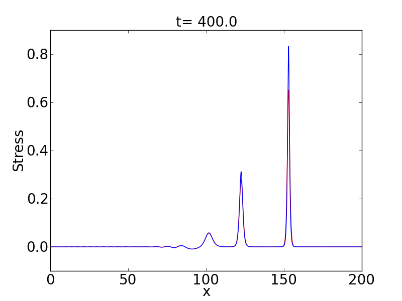
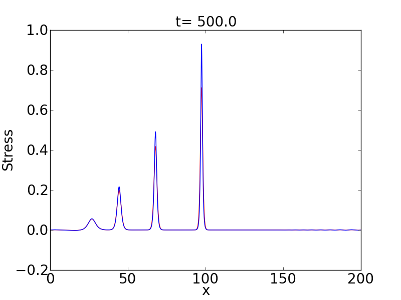
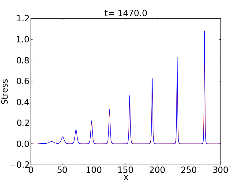
Note that the time and the domain I have to consider changes in each case. Obviously it is more expensive to obtain more and more solitary waves. This is because I need larger times and bigger domains to avoid interaction of the solitary waves.

Speed-amplitude relation

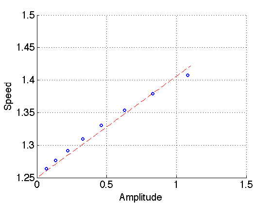
Considering the last plot; i.e., \(var=50\), I isolate the first eight c-solitary waves and propagate each for 100 seconds tracking the position of the maximum point in the stress. I use this information to estimate the speed of each c-solitary wave. Then we can do a linear least squares fitting as:

\(speed=1.25+slope*a,\)

where slope is the parameter to find. This is based on the fact (from homogenization theory) that small amplitude perturbations should propagate at the speed \(c_{eff}=1.25\). I did this fitting and get:

\(speed=1.25+0.1557*a,\)

which gives the figure below. Off course the higher amplitude solitary waves are influencing the fitting making it not to coincide with the small amplitude waves.

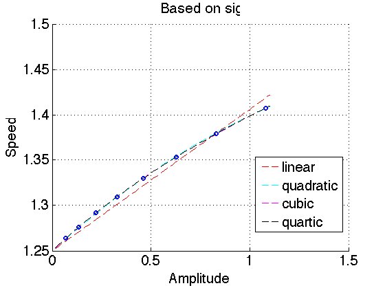
One can also do higher order least squares fitting. The following is a picture of curve fittings up to 4th order in \(a\). I think we are actually approximating the Talyor expansion of the amplitude-speed relation around \(a=0\).

Something else we can do is to approximate several derivatives around \(a=0\) (as many as c-solitary waves we have if we use a first order approximation) and then construct the corresponding truncated Taylor series. However, since the measurements of the speed-amplitude have some error I suppose the least squares fitting is the best option.

Speed-amplitude relation based on different amplitudes

So far I have been considering the stress to obtain the amplitude-speed relation. However, one can consider the amplitude of other variables such as the velocity or others.

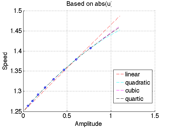
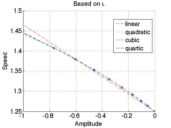
The following plots show the relation based on abs(u) and u. All of the fitting are of least-squares type and satisfy speed(0)=ceff.