c-scaling

In the following explanation I consider two c-solitary waves. The tallest one is refereed as sw1 and the shortest as sw2. Everything that has a 1 has to do with sw1 and likewise with sw2.

Let:

\(\begin{eqnarray*} a_1&=&\max_x(|u_1|),\\ a_2&=&\max_x(|u_2|), \end{eqnarray*}\)

each is a function of \(y\). What we discussed and see in the plots I have is that:

\(\begin{eqnarray*} \frac{1}{a_1}\sigma_1(\sqrt{a_1}(x-x_m) ) \approx \frac{1}{a_2}\sigma_2( \sqrt{a_2}(x-x_m) ) \\ \frac{1}{a_1}u_1(\sqrt{a_1}(x-x_m) ) \approx \frac{1}{a_2}u_2(\sqrt{a_2}(x-x_m) ) \end{eqnarray*}\)

For the velocity in \(y\), this is not quite the case. The following are surface plots of the scaled versions of \(v_1\) and \(v_2\) (using the same scaling). I also show a slice in y going through the maximum point.

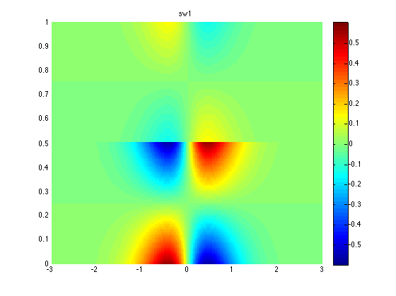
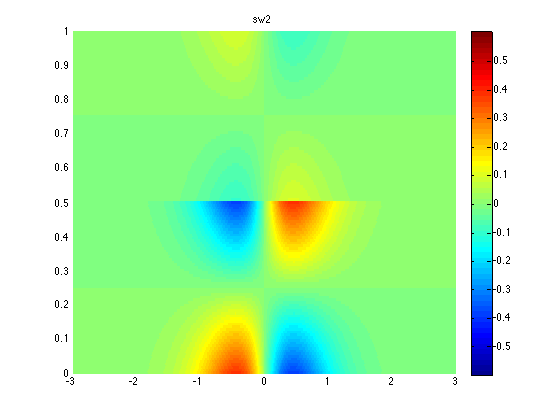
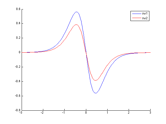
We can see the scaling is not very good in this case. I guess this may not be a very big deal and using solitary waves obtained form this scaling may still give good results after some energy gets thrown away.

Now the problem is that really this is not an scaling as in 1D; i.e., I can’t just take a solitary wave and scale it by an arbitrary constant. This is because \(a_1\) and \(a_2\) are really functions of \(y\) and they depend on each solitary wave. Say I have \(sw_2\) and I want to construct something close to \(sw_1\) from it. Even if I know the maximum amplitude of \(sw_1\), what I need to construct \(sw_1\) is \(a_1=a_1(y)\) which I obviously don’t know. The same is true to construct any solitary wave of higher amplitude; I need the corresponding \(a(y)\) function of the new solitary wave.

Now the question is if somehow knowing some characteristic of \(sw_1\) (the maximum value, the mean value or something else) I can construct \(a_1(y)\) from \(a_2(y)\) and such characteristic value.

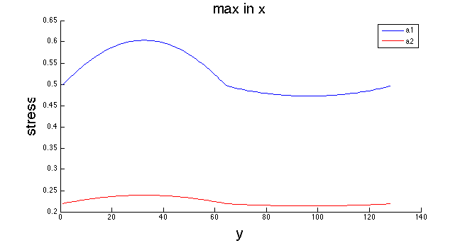
The following is a plot of \(a_1(y)\) and \(a_2(y)\). It is obvious there is no constant \(c\) such that \(a_1=c*a_2\).

However, if I shift them down by subtracting the mean value I can make them match. The following figure is a plot of \(a_1(y)-mean(a_1)\) and \(a_2(y)-mean(a_2)\).

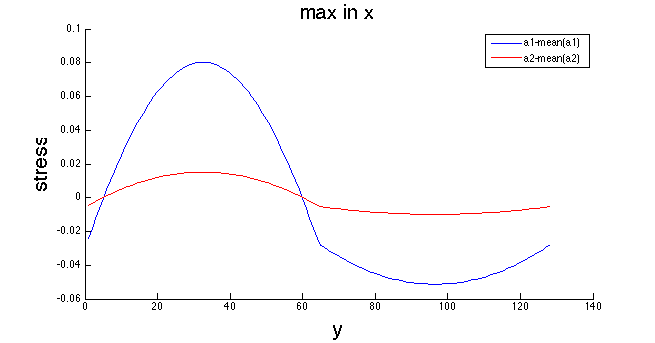
Now it seems feasible to scale \(a_2(y)-mean(a_2)\) to make it match with \(a_1(y)-mean(a_1)\).

NOTE: One can’t just take \(a_2(y)\) and multiply it by any number and construct form there a “solitary wave”. The result of that is most probably not going to be a solitary wave at all.

Matching the functions a(y)

As explained before for any solitary wave we need to construct the function \(a(y)=\max_x(|u|)\) from some characteristic value and the \(a(y)\) function from a different solitary wave. For this study I consider the first six solitary waves taken from the following figure.

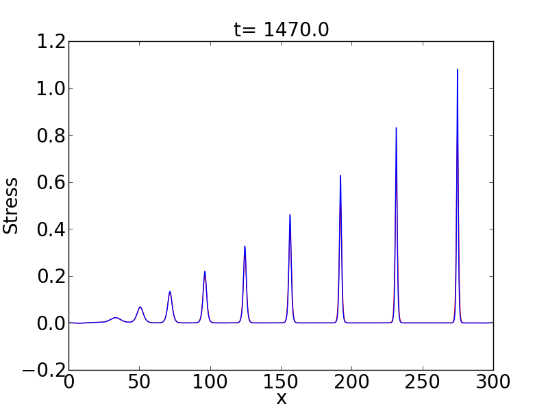
For each solitary wave I compute the corresponding \(a(y)\) function and plot \(\frac{1}{mean(a(y))^2}[a(y)-mean(a(y))]\).

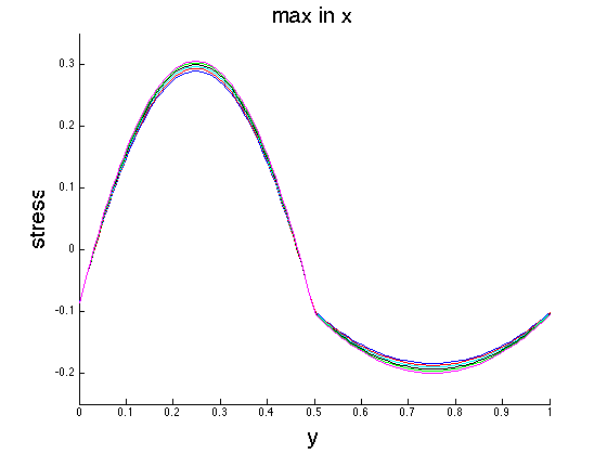
The agreement is fairly good. This means that given any solitary wave as reference one can construct the \(a(y)\) function for other solitary waves by knowing its mean. To check this, I construct \(a1\) from \(a2\). The following picture shows the original \(a1\) (solid line) vs the constructed one (dashed line).

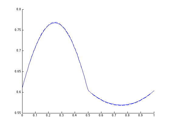
I can now construct nearly c-solitary waves of different amplitudes given any c-solitary wave.

Constructing nearly c-solitary waves

Now I will use the second c-solitary wave sw2 and, using the scaling explained before, construct waves close to sw1 and sw3 by just considering mean(a1(y)) and mean(a3(y)) respectively. Then I can see how good these nearly c-solitary waves are by comparing them with the actual sw1 and sw3.

The stress for sw1 and for the nearly sw1 is shown in the following picture.

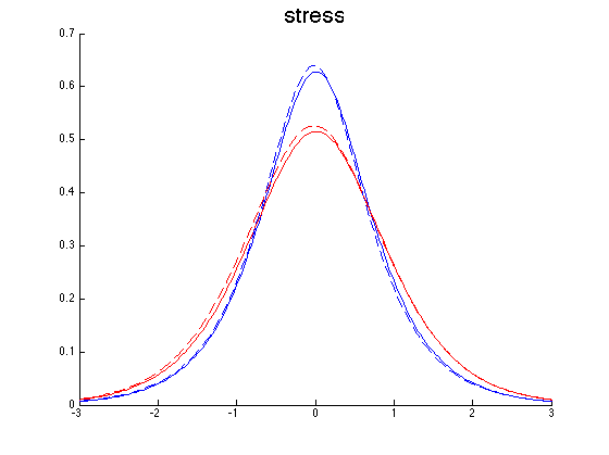
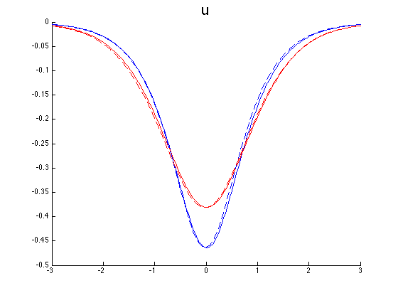
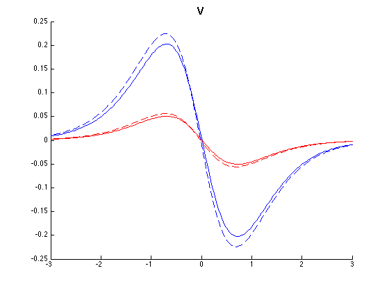
The next pictures show y-slices of the stress and the x-velocity at the middle of material A (blue) and B (red) and the y-velocity at the first (blue) and last (red) y-value. The solid line is the original sw1 and the dashed line is the constructed one. These y-slices in \(v\) are considered since \(v\) is almost zero at the middle of the materials. One can do a 2D interpolation and compute the relative errors, they are 2.8%, 2.5% and 8.9% for sigma, u and v respectively.

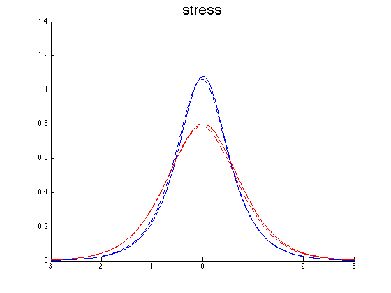
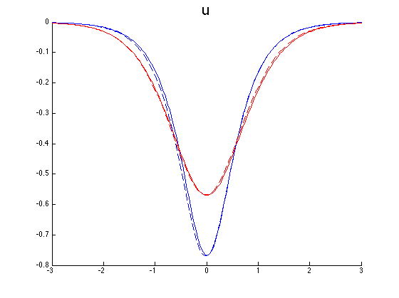
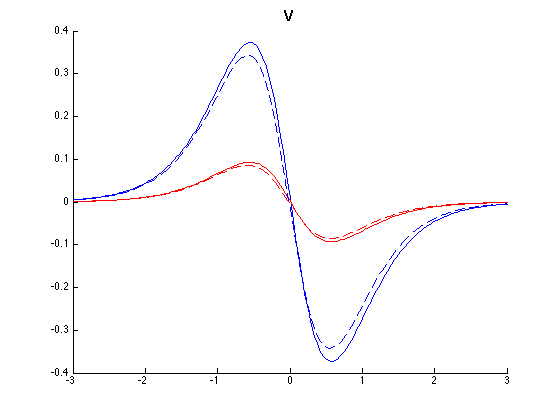
Now the next figure shows sw3 and the constructed sw3 from sw2.

The following pictures show the same slices as before but comparing now the original sw3 and the constructed one.